Parametric Equations and Polar Coordinates

Parametric Equations

So far, the graphs we have drawn are defined by one equation: a function with two variables, x and y . In some cases, though, it is useful to introduce a third variable, called a parameter, and express x and y in terms of the parameter. This results in two equations, called parametric equations.

Let f and g be continuous functions (functions whose graphs are unbroken curves) of the variable t . Let f (t) = x and g(t) = y . These equations are parametric equations, t is the parameter, and the points (f (t), g(t)) make up a plane curve. The parameter t must be restricted to a certain interval over which the functions f and g are defined.

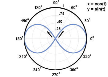
The parameter can have positive and negative values. Usually a plane curve is drawn as the value of the parameter increases. The direction of the plane curve as the parameter increases is called the orientation of the curve. The orientation of a plane curve can be represented by arrows drawn along the curve. Examine the graph below. It is defined by the parametric equations x = cos(t) , y = sin(t) , 0≤t < 2Π .

The curve is the same one defined by the rectangular equation x ² + y ² = 1 . It is the unit circle. Check the values of x and y at key points like t = , Π , and . Note the orientation of the curve: counterclockwise.

The unit circle is an example of a curve that can be easily drawn using parametric equations. One of the advantages of parametric equations is that they can be used to graph curves that are not functions, like the unit circle.

Another advantage of parametric equations is that the parameter can be used to represent something useful and therefore provide us with additional information about the graph. Often a plane curve is used to trace the motion of an object over a certain interval of time. Let's say that the position of a particle is given by the equations from above, x = cos(t) , y = sin(t) , 0 < t≤2Π , where t is time in seconds. The initial position of the particle (when t = 0 )is (cos(0), sin(0)) = (1, 0) . By plugging in the number of seconds for t , the position of the particle can be found at any time between 0 and 2Π seconds. Information like this could not be found if all that was known was the rectangular equation for the path of the particle, x ² + y ² = 1 .

It is useful to be able to convert between rectangular equations and parametric equations. Converting from rectangular to parametric can be complicated, and requires some creativity. Here we'll discuss how to convert from parametric to rectangular equations.

The process for converting parametric equations to a rectangular equation is commonly called eliminating the parameter. First, you must solve for the parameter in one equation. Then, substitute the rectangular expression for the parameter in the other equation, and simplify. Study the example below, in which the parametric equations x = 2t - 4 , y = t + 1 , - âàû < t < âàû are converted into a rectangular equation.

parametric

By solving for the parameter in one parametric equation and substituting in the other parametric equation, the equivalent rectangular equation was found.

One thing to note about parametric equations is that more than one pair of parametric equations can represent the same plane curve. Sometimes the orientation is different, and sometimes the starting point is different, but the graph may remain the same. When the parameter is time, different parametric equations can be used to trace the same curve at different speeds, for example.