What gives money value? We know that intrinsically, a dollar bill is just worthless paper and ink. However, the purchasing power of a dollar bill is much greater than that of another piece of paper of similar size. From where does this power originate?

Like most things in economics, there is a market for money. The supply of money in the money market comes from the Fed. The Fed has the power to adjust the money supply by increasing or decreasing the number of bills in circulation. Nobody else can make this policy decision. The demand for money in the money market comes from consumers.

The determinants of money demand are infinite. In general, consumers need money to purchase goods and services. If there is an ATM nearby or if credit cards are plentiful, consumers may demand less money at a given time than they would if cash were difficult to obtain. The most important variable in determining money demand is the average price level within the economy. If the average price level is high and goods and services tend to cost a significant amount of money, consumers will demand more money. If, on the other hand, the average price level is low and goods and services tend to cost little money, consumers will demand less money.

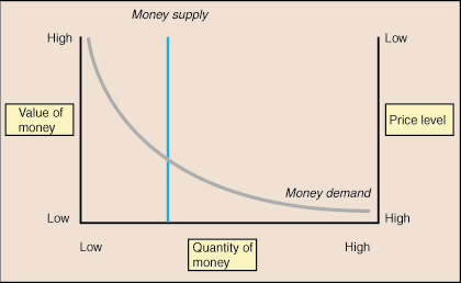
The value of money is ultimately determined by the intersection of the money supply, as controlled by the Fed, and money demand, as created by consumers. Figure 1 depicts the money market in a sample economy. The money supply curve is vertical because the Fed sets the amount of money available without consideration for the value of money. The money demand curve slopes downward because as the value of money decreases, consumers are forced to carry more money to make purchases because goods and services cost more money. Similarly, when the value of money is high, consumers demand little money because goods and services can be purchased for low prices. The intersection of the money supply curve and the money demand curve shows both the equilibrium value of money as well as the equilibrium price level.

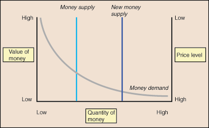
The value of money, as revealed by the money market, is variable. A change in money demand or a change in the money supply will yield a change in the value of money and in the price level. Notice that the change in the value of money and the change in the price level are of the same magnitude but in opposite directions. An increase in the money supply is depicted in Figure 2. Notice that the new intersection of the money supply curve and the money demand curve is at a lower value of money but a higher price level. This happens because more money is in circulation, so each bill becomes worth less. It takes more bills to purchase goods and services, and thus the price level increases accordingly.

The quantity theory of money is based directly on the changes brought about by an increase in the money supply. The quantity theory of money states that the value of money is based on the amount of money in the economy. Thus, according to the quantity theory of money, when the Fed increases the money supply, the value of money falls and the price level increases. In the SparkNote on inflation we learned that inflation is defined as an increase in the price level. Based on this definition, the quantity theory of money also states that growth in the money supply is the primary cause of inflation.

While the relationship between money supply, money demand, the price level, and the value of money presented above is accurate, it is a bit simplistic. In the real world economy, these factors are not connected as neatly as the quantity theory of money and the basic money market diagram present. Rather, a number of variables mediate the effects of changes in the money supply and money demand on the value of money and the price level.

The most important variable that mediates the effects of changes in the money supply is the velocity of money. Imagine that you purchase a hamburger. The waiter then takes the money that you spent and uses it to pay for his dry cleaning. The dry cleaner then takes that money and pays to have his car washed. This process continues until the bill is eventually taken out of circulation. In many cases, bills are not removed from circulation until many decades of service. In the end, a single bill will have facilitated many times its face value in purchases.

Velocity of money is defined simply as the rate at which money changes hands. If velocity is high, money is changing hands quickly, and a relatively small money supply can fund a relatively large amount of purchases. On the other hand, if velocity is low, then money is changing hands slowly, and it takes a much larger money supply to fund the same number of purchases.

As you might expect, the velocity of money is not constant. Instead, velocity changes as consumers' preferences change. It also changes as the value of money and the price level change. If the value of money is low, then the price level is high, and a larger number of bills must be used to fund purchases. Given a constant money supply, the velocity of money must increase to fund all of these purchases. Similarly, when the money supply shifts due to Fed policy, velocity can change. This change makes the value of money and the price level remain constant.

The relationship between velocity, the money supply, the price level, and output is represented by the equation M * V = P * Y where M is the money supply, V is the velocity, P is the price level, and Y is the quantity of output. P * Y, the price level multiplied by the quantity of output, gives the nominal GDP. This equation can thus be rearranged as V = (nominal GDP) / M. Conceptually, this equation means that for a given level of nominal GDP, a smaller money supply will result in money needing to change hands more quickly to facilitate the total purchases, which causes increased velocity.

The equation for the velocity of money, while useful in its original form, can be converted to a percentage change formula for easier calculations. In this case, the equation becomes (percent change in the money supply) + (percent change in velocity) = (percent change in the price level) + (percent change in output). The percentage change formula aids calculations that involve this equation by ensuring that all variables are in common units.

The velocity equation can be used to find the effects that changes in velocity, price level, or money supply have on each other. When making these calculations, remember that in the short run, output (Y), is fixed, as time is required for the quantity of output to change.

Let's try an example. What is the effect of a 3% increase in the money supply on the price level, given that output and velocity remain relatively constant? The equation used to solve this problem is (percent change in the money supply) + (percent change in velocity) = (percent change in the price level) + (percent change in output). Substituting in the values from the problem we get 3% + 0% = x% + 0%. In this case, a 3% increase in the money supple results in a 3% increase in the price level. Remember that a 3% increase in the price level means that inflation was 3%.

In the long run, the equation for velocity becomes even more useful. In fact, the equation shows that increases in the money supply by the Fed tend to cause increases in the price level and therefore inflation, even though the effects of the Fed's policy is slightly dampened by changes in velocity. This results a number of factors. First, in the long run, velocity, V, is relatively constant because people's spending habits are not quick to change. Similarly, the quantity of output, Y, is not affected by the actions of the Fed since it is based on the amount of production, not the value of the stuff produced. This means that the percent change in the money supply equals the percent change in the price level since the percent change in velocity and percent change in output are both equal to zero. Thus, we see how an increase in the money supply by the Fed causes inflation.

Let's try another example. What is the effect of a 5% increase in the money supply on inflation? Again, we being by using the equation (percent change in the money supply) + (percent change in velocity) = (percent change in the price level) + (percent change in output). Remember that in the long run, output not affected by the Fed's actions and velocity remains relatively constant. Thus, the equation becomes 5% + 0% = x% + 0%. In this case, a 5% increase in the money supply results in a 5% increase in inflation.

The velocity of money equation represents the heart of the quantity theory of money. By understanding how velocity mitigates the actions of the Fed in the long run and in the short run, we can gain a thorough understanding of the value of money and inflation.