|
||||||||||||||||||||||||||||||||||||||||||||||||
|
||||||||||||||||||||||||||||||||||||||||||||||||
|
Home : Other Subjects : Economics Study Guides : Microeconomics : Supply & Demand : Demand : Utility
Utility
Utility and Indifference Curves
We know how to represent changes in demand as price or income
changes on a graph, but how can we show preferences? What makes buyers
happy and how can we measure that happiness? Economists use the term
utility when referring to the level of happiness or satisfaction
that someone experiences from buying (or selling) goods and services:
the more utility, the happier the person. Utility is typically
represented on a graph in an indifference curve. An indifference
curve represents all of the different combinations of two goods that
generate the same level of utility. What this means is that each point
on an indifference curve represents a combination of goods. All points
on one indifference curve give the person the exact same amount of
happiness. For instance, if you give Jim a choice between points A and
B on this indifference curve, he won't really mind either way, he is
indifferent. One shirt and two hats makes him just as happy as two
shirts and one hat, which is why both points are on the same indifference curve.
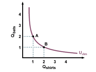
In general, indifference curves bow in towards the origin, rather
than being straight lines or outward-bulging curves. The reason for
this is that most people do not like extremes: they would rather have a
some shirts and some hats than many hats and no shirts. This changing
preference results in the traditional inward-curving indifference
curves, and illustrates the effects of diminishing returns. In
this example, diminishing returns simply means that the first hat Jim
gets makes him happier than the second hat, which makes him happier
than the third, and so on. His marginal utility--the extra utility he gets
with each hat--decreases with the number of hats he gets. After a while, he has
had enough of hats, the extra ones don't make him much happier, and he'd rather
get a shirt, and might even trade several hats for one shirt. Generally, at
the extremes, people are willing to give up many hats to get a few
shirts; as the numbers even out, this swapping ratio decreases, and
then when they start moving to the other extreme, they want a lot of
shirts in exchange for any hats they might give up.
Another example that illustrates the principle of diminishing returns would be
the case in which you give Thom a choice between gold and steak. We all know
that a bar of gold is worth more than a steak, so only a fool would choose the
steak over the gold, right? Thom knows this. If you ask Thom to choose between
a bar of gold and a steak, he will probably choose the gold, and be very excited
to have a bar of gold. The marginal utility of that first bar of gold is quite
high. An hour later, he will choose another bar of gold, and he will still be
happy to get another bar of gold; the marginal utility he gets from the second
bar of gold might not be quite as high as the marginal utility from the first
bar, but it's still higher than the marginal utility he would get from a steak.
This will continue, bar after bar, with the added utility of each bar of gold
being a little lower than the last. Eventually, Thom will start to get hungry,
and if he gets hungry enough, then he will choose the steak over the gold, as
the marginal utility from the steak will be higher than the marginal utility
from a bar of gold. Thom still knows the relative values of gold and steak, and
he knows that he is choosing something that is worth less, but in his situation,
he has so much gold that more gold makes very little difference, but a steak can
make a large difference, as he is very hungry.
Different indifference curves represent different levels of
utility, and in general, more is better: the more goods you have, the
happier you are. On the graph, we see this preference for more as an
indifference curve that is further away from the origin. Thus,
because curve 2 is further out than curve 1, and represents a higher
level of utility, any point on curve 2 will be preferable to
any point on curve 1, and any point on curve 3 will be
preferable to any point on curves 1 or 2.
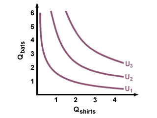
![]() Indifference Curves
A few more important observations about one person's indifference
curves: they can never cross. Why is this true? Think about it
this way: if curve 2 is supposed to make you happier than curve 1, but
curve two crosses curve 1, then that means that at the point of
intersection, you are experiencing two different levels of utility,
that is, you are both happy and happier at the same time, which makes
no sense. Thus, indifference curves never intersect, but move further
away from the origin with increased levels of utility.
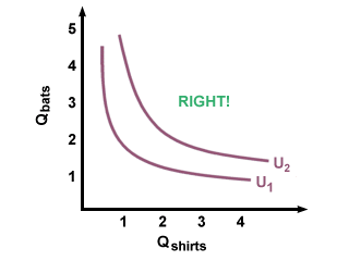
![]() A Correct Set of Indifference Curves ![]() An Incorrect Set of Indifference Curves
The indifference curves we have been considering are for normal
goods. How can we tell? Because more of either good increases
utility. Starting on curve 1 and moving outwards (increasing the
number of hats) or upwards (increasing the number of shirts) lands us
on curve 2, representing a higher level of utility. Using different
types of goods changes what indifference curves look like.
For instance, if one good is a normal good, such as CDs, and the
other good is an undesirable good, such as Spam, the indifference
curves will look like this, with the second indifference curve being better
than the first:
Utility Curves for Normal and Undesirable Goods
What if the consumer doesn't care about one of the goods, meaning
that getting more or less of that good doesn't make them happier or
unhappier? For instance, replace the Spam with expired baseball
tickets. Jim likes getting CDs, but really doesn't care how many
expired baseball tickets he gets. This makes his indifference curves
look like this:
Indifference Curves for Normal and Neutral Goods
Another instance in which indifference curves behave strangely is in
the case of complementary goods. Demand for complementary goods is
directly related. In other words, buying one good increases the probability
you'll buy the other good, those two goods are complementary. Mittens are an
extreme example of complementary goods: if you buy a right mitten, it
is almost a sure bet that you'll buy a left mitten. This also means
that having extra stray mittens isn't likely to increase your utility.
There is virtually no difference in your happiness whether you have one
right mitten and one left mitten, or two right mittens and one left
mitten. This shows up in the following indifference curves (note that
only a simultaneous increase of right and left mittens will result in
increased utility).
What if the two goods being evaluated are pretty much the same?
Such goods are called substitute goods: the buyer considers them to
be interchangeable. One example of perfect substitutes (though some
might argue otherwise) could be Coke and Pepsi. If you consider them
to be the same thing, then you don't mind which one you get. More is
still better, but you don't care what combination of the two you get,
which means that when you have a lot of Pepsi, you would not be willing
to trade three cans of Pepsi for one can of Coke, eliminating the
inward bend of the indifference curves. This results in indifference
curves like this:
Utility Optimization
While it is impossible to know exactly what goes on inside a
buyer's head while they are making a decision, we can assume that a
normal person will choose whichever combination will make them as happy
as possible, given their choices and their budget. On the graph, this
means that they will choose whichever combination lands them on the
highest indifference curve possible. We can see this optimization if we
draw in the consumer's budget constraint on the same graph as the
consumer's indifference curves.
To draw a budget constraint, a line that shows the maximum amount
of goods a buyer can purchase with their available funds, you need to
know two things: 1) how much money they have, and 2) the prices of the
two goods being considered. Once you have both pieces of information,
it is simply a matter of finding out the maximum amount of the first
good you can buy, without buying any of the second, then finding the
maximum amount of the second good you can buy, without buying any of
the first. Mark these points on the graph and connect them. To
illustrate, suppose Tina has $100. She is deciding how many bottles of
wine and how many wine glasses she wants to buy. If wine costs $20 a
bottle and glasses cost $5 each, then the most wine she can buy is
($100/$20)=5 bottles. Likewise, she can buy at most ($100/$5)=20 wine
glasses. Her budget constraint would look like the darker line, while
the filled area includes all of her possible buying decisions, given
the amount of money she has. Anything not included in the colored area
is out of her budget:
![]() Tina's Budget Constraint
If we know her indifference curves, we can draw her budget constraint
in with them on the same graph. After that, it is simply a matter of
finding the outermost indifference curve that is tangent to (just
barely touches) her budget constraint, and use this tangent point as
her optimal combination of wine and glasses. In this case, it is the
second indifference curve that optimizes her utility given her budget.
It looks like Tina will buy about 12 wine glasses and 2 bottles of
wine. Even though the optimal amount is a little more than 2 bottles,
she has to buy either 2 bottles or 3 bottles, and 2 is all she can
afford. (When doing such problems, never round up, since that will
land you outside of the budget constraints).
Why does it have to be the indifference curve that is tangent to
her budget constraint? If it were an indifference curve that crosses
her budget constraint, such as the first indifference curve, then we can see
that the two points of intersection don't make her as happy as the
single tangent point in the previous graph. By picking the outermost
curve that still touches her budget constraint, we have maximized her
utility. We can't pick a curve any further out, such as the third
indifference curve, since she can't afford to buy more than $100 worth
of wine and glasses.
Obviously, budget constraints change with changes in income or
price. For instance, if Tina now has $125 instead of $100, her new
budget constraint will be a parallel shift out from her original budget
constraint. The yellow shaded region represents the increase in
possible purchases she can make:
![]() A Shift in Tina's Budget Constraint
On the other hand, if Tina still has only $100, but the price of
wine changes from $20 a bottle to $10 a bottle, her budget constraint
will pivot to reflect this change:
![]() A Pivot in Tina's Budget Constraint |
|
|||||||||||||||||||||||||||||||||||||||||||||||
|
|
|||||||||||||||||||||||||||||||||||||||||||||||
|
Contact Us | Privacy Policy | Terms and Conditions | About
©2006 SparkNotes LLC, All Rights Reserved.
|
||||||||||||||||||||||||||||||||||||||||||||||||