The Graphical Approach
By now, we are familiar with graphs of supply curves and demand curves.
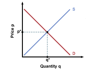
To find market equilibrium, we combine the two curves onto one graph. The
point of intersection of supply and demand marks the point of equilibrium.
Unless interfered with, the market will settle at this price and quantity. Why
is this? At this point of intersection, buyers and sellers agree on
both price and quantity. For instance, in the graph below, we see that at the
equilibrium price p*, buyers want to buy exactly the same amount that sellers
want to sell.


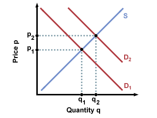
We can also see what happens when one of the curves shifts up or down in
response to outside factors. For example, if we were to look at the market for
Beanie Babies before and after they became a popular fad, we would see a shift
outwards from the initial demand curve over time. The reason for this is that
as people began to like Beanie Babies, their preferences changed, and they began
to want Beanie Babies enough that they would pay much more for each Beanie Baby
than they would have previously. We can see this new preference for Beanie
Babies in the outward shift of the demand curve: for every price, buyers will
buy more Beanie Babies than they would have before the fad.

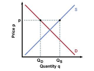
It is only through a shift in either the supply or the demand curve that the market equilibrium will change. Why is this? If neither curve shifts, and we move along one of the curves, the market will naturally shift back to equilibrium. For example, if we look at a market in equilibrium, and a store tries to move up its supply curve by selling goods at a higher price, the result will be that no one will buy the goods, since they are less expensive at the store's competitors. The store will have to either go out of business, or move its prices back down to equilibrium.
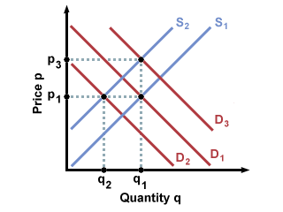
What happens if both curves shift? Will we end up at the same equilibrium
point? In this model, it is not possible to reach the same equilibrium: either
the price or the quantity can be the same as the previous equilibrium, but not
both, unless the curves shift back to their original positions. To illustrate
why this is true, consider the graph below. The initial equilibrium, between
supply curve 1 and demand curve 1, has price p* and quantity q*. If supply
shifts to supply curve 2, both equilibrium price and quantity change. It is now
possible to change back to our original price by shifting the demand curve to
position 2 or it is possible to revert to our original quantity by
shifting the demand curve to position 3. Note that we cannot reach the original
equilibrium point unless we move the curves back to their original points.

The Algebraic Approach
We have worked with supply and demand equations separately, but they can also be combined to find market equilibrium. We have already established that at equilibrium, there is one price, and one quantity, on which both the buyers and the sellers agree. Graphically, we see that as a single intersection of two curves. Mathematically, we will see it as the result of setting the two equations equal in order to find equilibrium price and quantity.
If we are looking at the market for cans of paint, for instance, and we know that the supply equation is as follows:
QS = -5 + 2PAnd the demand equation is:
QD = 10 - PThen to find the equilibrium point, we set the two equations equal. Notice that quantity is on the left-hand side of both equations. Because quantity supplied is equal to quantity demanded at equilibrium, we can set the right-hand sides of the two equations equal.
QS = QDAt equilibrium, paint will cost $5 a can. To find out the equilibrium quantity, we can just plug the equilibrium price into either equation and solve for Q.
-5 + 2P = 10 - P
3P = 15
P = 5
Q* = QS
QS = -5 + 2(5)
QS = Q* = 5 cans
Shifts up and down supply and demand curves are represented by plugging different prices into the supply and demand equations: different prices yield different quantities. For example, changing the price to $6 a can would decrease quantity demanded from 5 cans to 4 cans, as we can see when we plug the two prices into the demand function:
P = 5The equivalent of shifting supply and demand curves is changing the actual supply and demand equations. Let's say that everyone in a small town just recently painted their houses, and therefore no longer need any paint. This means that they will be less willing to buy paint, even if the price doesn't go up. Their new demand function might be:
QD = 10 - 5 = 5 cans
P = 6
QD = 10 - 6 = 4 cans
QD = 7 - PWe can see that for any price, they will demand fewer cans of paint. At the old equilibrium price of $5, they will only buy:
QD = 7 - 5 = 2 cans of paint
This new equation, representing a shift in demand, also causes a shift in market equilibrium, which we can find by setting the new demand equation equal to supply:
QS = QDNow to solve for the equilibrium quantity:
-5 + 2P = 7 - P
3P = 12
P = $4 a can
Q* = QSAt the new equilibrium, 3 cans of paint will be sold at $4 each.
QS = -5 + 2P = -5 + 2(4)
QS = Q* = 3 cans of paint


 payment page


