


Like the market for any other good, the market for money settles into an equilibrium where quantity supplied equals quantity demanded. In a graphical analysis, both the equilibrium quantity of money lent (\(q^*\)) and the equilibrium interest rate (\(r^*\)) are given by the point where the supply and demand curves intersect:
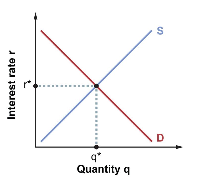
Suppose that the interest rate is initially greater than \(r^*\). Lenders will quickly learn, from the lack of interest on the part of borrowers, that they have set the lending rate too high. They will come down in order to attract more borrowers. On the flip side, if the interest rate is initially less than \(r^*\), lenders will be inundated with requests to borrow and will realize they can charge more interest and still lend out as much money as they’re prepared to supply.
Now suppose some new industry is picking up steam and firms in that industry want to build more production facilities. As they start filing more applications for loans to fund the construction projects, the demand curve shifts to the right:
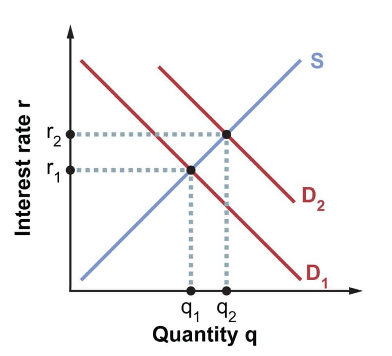
The total quantity of money lent out will increase, and the rate at which it is lent out will go up. In similarly predictable fashion, a decrease in the demand for loans (a leftward shift of the demand curve) will cause both the quantity and rate to go down.