


Another way the government can reshape a market is through taxes. Suppose we’re talking about a tax on potato chips, $1 per bag, and this tax is paid by the sellers. In the figure below, the market equilibrium without the tax would be at quantity \(q_1\) and price \(p_1\). When the tax is imposed, the supply curve \(S_1\) reflects how much sellers are willing to supply at every price based on what they keep as revenue, after paying the tax. The other supply curve, \(S_\text{tax}\), reflects what buyers pay, \(p_\text{tax}\), namely the seller’s revenue plus the $1 tax. This curve lies higher than \(S_1\) by a distance of $1 at every point. So the imposition of tax on sellers causes a vertical shift of the supply curve, by a distance equal to the amount of the tax.

The Tax Burden
With the tax, the market equilibrium is at quantity \(q_\text{tax}\) and price \(p_\text{tax}\). Notice that although legally the burden is on the suppliers to pay the tax, economically the price increase at the point of sale shifts some, but not all, of the tax burden onto consumers: \(p_\text{tax}\) is higher than price \(p_1\), but not by a full $1.
The effect would in principle be the same if the government somehow managed to collect the tax from consumers instead of sellers. (This would be cumbersome in practice.) Then the demand curve would shift downward a distance of $1, to reflect what buyers were willing to pay sellers given that the buyers would also be paying the government $1 per bag of chips. The equilibrium price at the point of sale would be lower, but not a full $1 lower, than the no-tax equilibrium price \(p_1\).
Effect on Social Welfare
Without the tax, the total surplus generated by the market is represented by the area between curves \(D\) and \(S_1\) to the left of the equilibrium point. The area above the horizontal line at \(p_1\) is the consumer surplus; the area below \(p_1\) is the producer surplus. With the tax, the total surplus is divided into three parts, not two, as shown below.
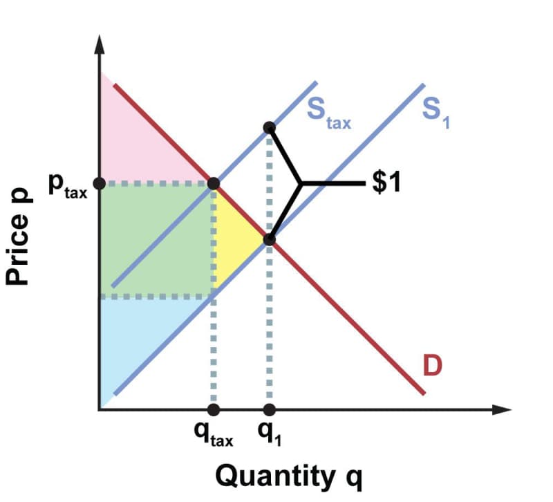
Both the consumer surplus, shown in pink, and the consumer surplus, shown in blue, are now considerably smaller. Between them lies a green rectangle whose area represents the government’s tax revenue: the number of units sold, \(q_\text{tax}\) (the base of the rectangle) times the tax per unit, in this case $1 (the height of the rectangle). Notice that this area will be very small when the tax is small. As the tax increases, the green area will grow larger, but if the tax continues to increase, the green area starts shrinking again. A big enough tax will drive \(q_\text{tax}\) to zero, at which point consumer surplus, producer surplus, and government tax revenue are all zero. Somewhere between the extremes is a “sweet spot” that maximizes tax revenue.
The total surplus is now consumer surplus + producer surplus + tax. What about the yellow triangle? That represents deadweight loss: social welfare that was present before the tax but with the tax is no longer available to anyone—not to consumers, nor producers, nor the government. The basic cause of deadweight loss is simply that the amount of trade has been reduced, from \(q_1\) to \(q_\text{tax}\), and with less trade there are fewer gains from trade. This is a natural effect of any tax imposed on trade. Occasionally, a reduction in trade may be desirable (think of a tax on cigarettes, for example), but taxes do not care about the nature of the good in question. The trade-discouraging effect of taxes applies across the board.
From a policy perspective, then, taxes involve a trade-off. A certain level of taxation is necessary to fund government. And up to a point, at least, higher taxes mean more money for government. But at every point, more taxes mean less total welfare, even when government tax revenue is included in that total.
Elasticity Effects
Regardless of who pays the tax, economically the burden of a tax is shared between buyers and sellers. But how the burden is distributed depends on the elasticities of demand and supply. Suppose that demand for potato chips becomes less elastic for some reason. We can model this by rotating the demand curve counterclockwise about the equilibrium point:
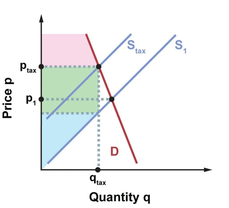
Note that ptax increases, so that the difference \(p_\text{tax} - p_1\) , which is the share of the tax that ends up coming out of the buyer’s pocket, is greater than before, and the seller’s share is less. This illustrates a general principle: when a tax is imposed, the tax burden tends to fall more heavily on buyers with inelastic demand than on buyers with elastic demand. Similarly, the tax burden tends to fall more heavily on sellers with inelastic supply than on sellers with elastic supply. (We would demonstrate this by rotating the supply curves instead of the demand curve.)