As with demand, it is also possible to model supply using equations. These supply equations, or supply functions, are used to numerically represent firm behavior and the variation of firm behavior with price. For simplicity's sake, we will again use simple algebraic equations.
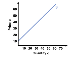
Suppose Amy's bookstore sells textbooks with a supply curve that looks like this:

The corresponding equation that describes the bookstore's supply of textbooks will be the equation for the line:
\(q = -10 + p\)
If we want to see how many books the store is willing to sell if the price is $50, we plug 50 in for p and solve for q. In this case,
\(q = -10 + 50 = 40\) textbooks
If we want to solve for market supply using the algebraic approach instead of the graphical approach, we just add the supply equations together. Suppose the equation for Tony’s bookstore supply is \(q = –5 + 1.5p\). Then adding Amy's bookstore's supply to Tony's bookstore's supply looks like this:
\(q = –10 + p\)
+ \(q = –5 + 1.5p\)
––––––––––––––
\(q = –15 + 2.5p\)
If price is still equal to $50, we find out that together, Amy and Tony will sell:
\(q = -15 + 2.5(50) = 110\) textbooks
The caveat about using horizontal addition to find demand quantities also applies to horizontal addition to find supply quantities: it only works when the quantities from the individual suppliers’ equations are all non-negative. For instance, the supply equation for Amy's bookstore will give a negative quantity supplied if the price is under $10 per textbook. Since it is impossible to supply a negative quantity of textbooks, for values under $10 Amy’s store will zero 0 textbooks. Before adding together two or more supply equations, always check to make sure that none of them will give you negative results for the price you’re plugging in.


