


A monopoly market is characterized by the following conditions:
- One supplier, the monopolist
- No close substitute to the output good
- No threat of competition
These conditions usually result in very high prices, since there is no competition to keep prices in check. For example, Pepsi and Coke cost about the same amount of money. If Pepsi were to charge twice as much, most people would choose to buy Coke or some other cola, such as RC or Shasta, and Pepsi would lose business and revenue. However, if Coke and the other non-Pepsi colas did not exist, Pepsi would be a price maker, exerting control over the market price. In other words, it would have market power. The firm could charge twice as much as it currently does. With no substitutes available, people would buy Pepsi at the higher price, and Pepsi would have a huge profit margin.
To see in detail how this plays out, we can model the workings of monopolies both graphically and algebraically. We start with a graphical analysis.
The Graphical Approach
The profit-maximizing rule for any firm, regardless of the type of market, is that output volume should be adjusted to make marginal revenue equal marginal cost: \(MR = MC\). In a competitive market, the demand curve for any one firm’s output is horizontal at the constant price level, so that \(D = AR = MR = p\).
To maximize profit, then, a firm simply finds the intersection of its \(MC\) curve with the horizontal demand curve. (The firm’s \(MC\)curve, by the way, is its individual supply curve, because in a competitive market the \(MC\) curve marks, for every additional unit, the minimum price the firm needs to receive for that unit, in order to cover the cost of producing it.)

Monopolists face the more familiar, downward-sloping demand curve for their product, because the market demand curve and the demand curve for the monopolist’s output are one and the same. This makes it more difficult to find the point where \(MR = MC\), because the monopolist’s marginal revenue is not fixed at constant market price \(p\), like the marginal revenue in a competitive market.
By way of example, let's take another look at Pepsi-as-a-monopolist. As a sole supplier, Pepsi could try selling its cola at $10,000 a can. It might be able to sell one can. The marginal revenue on that first can is $10,000. To sell two cans, however, Pepsi might have to lower its price to $7000 a can, for a total revenue of $14,000. The marginal revenue on the second can is $14,000 – $10,000 = $4,000, which is quite a bit less than $10,000. As Pepsi sells more and more cans of soda, the marginal revenue continues to drop.
Monopolists will find their profit-maximizing point by finding the intersection between their downward-sloping \(MR\) curve and their \(MC\) curve. Note that in a monopoly market, the \(MR\) curve does not coincide with demand curve \(D\), so the profit-maximizing point chosen by a monopolist results in higher prices and lower consumption than in a competitive market.

Monopolists are able to sell their products at well above their average total cost, thereby earning much higher profits than competitive firms:

The Algebraic Approach
Assume that a monopolistic firm faces a linear, downward- sloping market demand curve, described as follows:
\(q = 100 - p\)
Let's further assume its marginal cost curve is constant at a value of 10.
\(MC = 10\)
Our firm naturally wants to maximize profits and will therefore aim to satisfy the profit maximizing condition, \(MC = MR\). Marginal costs are constant at 10, so half of our equation is easy. To find our marginal revenue, we first look at the total revenue. Total revenue is simply \(R = pq\). (This equation does not assume that \(p\) is constant, only that all units sell at the same price, whatever it is.) If we rewrite the demand equation to make \(p\) a function of \(q\),
\(p = 100 - q\),
we can then rewrite our total revenue as:
\(R = (100-q)q = 100q - q^2\)
The marginal revenue is simply the first derivative of the total revenue with respect to \(q\).
\(MR = 100 - 2q\)
Derivatives are a calculus concept. If you don't feel comfortable with derivatives, you can convince yourself of this formula for \(MR\) by analyzing its components.
\(MR = (100 - q) - q\)
\(100 - q\) is the price according to our market demand curve. This \(100 - q\) represents the marginal revenue brought in by selling the next unit. However, in order to sell the next unit, we had to lower the price by 1 for all units sold (the demand curve has a slope of –1, so the tradeoff between \(q\) and \(p\) is 1 for 1.) Therefore, on the margin, we lost 1 unit of revenue for each of the q units sold. The marginal revenue is then:
\((100-q)-q = 100 - 2q\)
To solve for the monopolistic equilibrium, we find the quantity at which \(MR = MC\):
\(100 - 2q = 10 \\q= 45\)
At this quantity, the market price would be \(100-45=55\). Assuming no fixed costs, the profits for this firm would be \(45 × (55 − 10) = 2025\). Naturally, this is a vast improvement for the firm over the competitive outcome of zero profits.
Natural Monopolies
In general, true monopolies are rare. For instance, a supermarket may be the only food supplier in a particular town, but if it raises its prices and retains too much of a profit, a competitor is liable to enter the space. Even the threat of serious competition entering the market forces the existing firm to act with moderation, differently from how it would act if it didn’t need to fear competition at all.
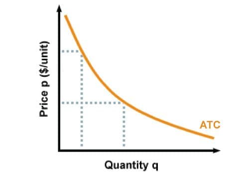
For certain kinds of goods, however, monopoly markets arise naturally. The key is the shape of the average total cost (\(ATC\)) curve. Typically, the \(ATC\) curve is U-shaped; that is, average total cost starts to rise as output grows large enough. (See the chapter on Firm’s Profit.) If instead the \(ATC\) continues to slope downward, then it is likely that a natural monopoly will form.
Why is this true? Any firm that establishes itself in this kind of environment enjoys unlimited economies of scale and therefore is able to drive away smaller competitors. Let's say that in the market for computers, Eliot Computer Lab ("ECL") gets a head-start on production and has already made 1000 units before its competitors get started. At that point, ELC has a much lower average cost than the new firms, and therefore has a significant advantage over its competitors, since it can charge lower prices and make more profits. If it ever feels threatened by new firms, it can increase production and lower the price even more, so that the new firms cannot compete, since they are still further back on the cost curve. In such a case, ECL would be a natural monopolist, and other firms would exit the market.