


In the labor market, demand comes from firms and supply comes from households. The combination of supply and demand curves for labor determines how much labor is purchased, and at what price. The unit price of labor is usually called a wage.
Because the theory of the supply of labor is related to the theory of individual choice, labor supply is left for the Preference and Choice chapter. Here, we will focus on labor demand before considering the equilibrium produced by supply and demand.
Labor Demand
Firms need workers to make products, design those products, package them, sell them, advertise for them, ship them, and distribute them, among other tasks. No worker will do this for free, so firms must enter into the labor market and buy labor. Firms determine the amount of labor they demand according to several considerations: how much the labor will cost (as represented by the market wage), and how much they feel they need, much in the way that buyers in the goods and services market buy according to the market price and their own needs.
Marginal Revenue Product of Labor
However much labor a firm is currently using, the marginal product (\(MP\)) of labor is the increase in production output quantity that would be achieved by adding one more unit of labor. The additional labor unit may be thought of as an additional worker or as an additional hour of work, so long as the wage, \(w\), is handled in the same way, either as an additional worker’s salary or as an hourly wage. If we multiply the \(MP\) by the market price, \(p\), of a unit of output, we obtain the marginal revenue product (\(MRP\)) of labor:
\(MRP=MP×p\)
This is the extra revenue a firm generates when it buys one more unit of labor. As long as the \(MRP\) of labor exceeds the wage, \(w\), paid for that extra labor, a firm will be willing to pay for more labor in order to increase output. The extra labor is worth the cost. If the \(MRP\) of labor is less than the market wage, on the other hand, then the firm is using too much labor, and it will probably cut back. If the \(MRP\) of labor is equal to the market wage, the firm is at its optimal point of labor consumption. To sum up,
\(MRP > w\): The firm will buy more labor
\(MRP = w\): The firm is buying the right amount of labor
\(MRP < w\): The firm is buying too much labor
The Law of Diminishing of Returns
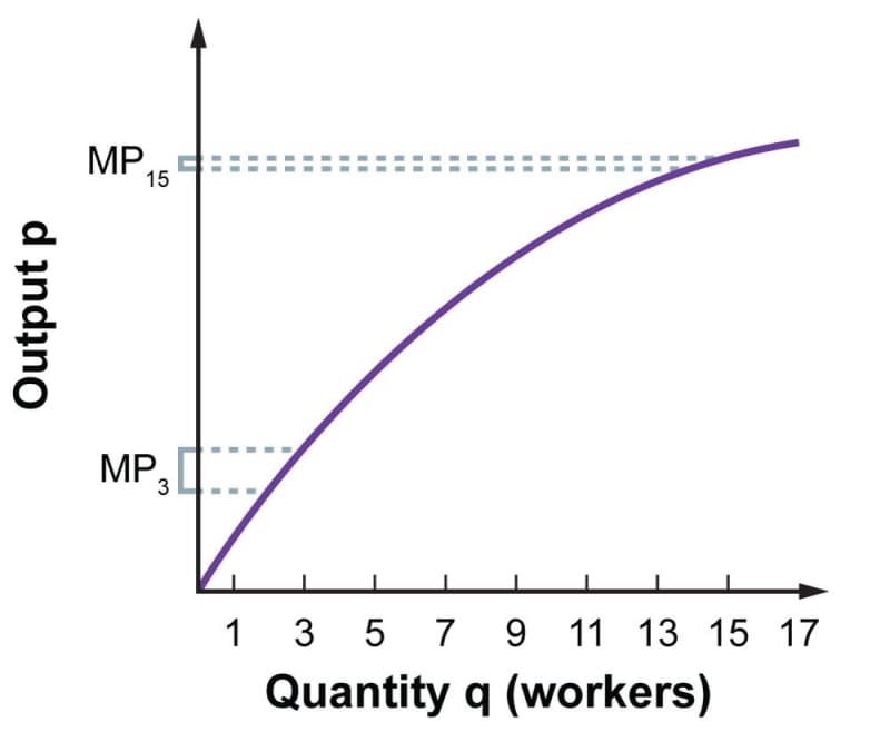
The reason the \(MRP\) of labor varies is the law of diminishing returns. When a firm is hiring and is deciding how many workers it needs, it knows that the first worker added will make the biggest difference. For a while, every additional worker will yield a large marginal product (\(MP\)). However, at some point additional workers will start to yield less in the way of added output. Economists picture this phenomenon using a production function that levels off as the number of workers increases. Note that \(MP_\text{15}\), the \(MP\) of the 15th worker, is smaller than \(MP_3\), the \(MP\) of the 3rd worker:
The reason for the decline in the marginal product is that after a certain point, additional workers have a hard time being as productive as their predecessors. Imagine, for instance, that a small furniture store is hiring workers. One worker will get a good deal done on their own. The second worker will probably be productive, as well. The sixteenth worker, however, would probably get nothing done, since there wouldn't be enough space or tools to make furniture.
If we graph the marginal product of each worker instead of the total output, then between the second and the sixteenth worker, we see a gradual drop in marginal productivity: additional workers may add to productivity, but each new worker contributes less, until the marginal product (\(MP\)) is 0. Because \(MRP=MP×p\), the decline in MP is mirrored by a decline in \(MRP\):

We get a similar effect if we keep the number of workers the same but ask each worker to work longer hours at the same hourly pay rate. Part-time workers may happily accept an increase in hours, but as workers’ hours increase, workers’ enthusiasm starts to drops off, and with it their efficiency.
Because at every hiring level the \(MRP\) represents what an additional unit of labor is worth to the firm and therefore the wages it would be willing to pay for that unit, we can treat the curve representing the \(MRP\) of labor as the firm’s labor demand curve. The point along the \(MRP\) curve where the \(MRP\) of labor equals the wage prevailing in the labor market as a whole (in the firm’s industry, for the kind of worker in question) determines how much labor a firm is willing to hire. For our imaginary furniture store, the situation might look like this:

The horizontal line at \(w\) serves as the labor supply curve. (Labor supply is perfectly elastic from the perspective of an individual firm, because the market wage rate does not change appreciably based on the number of people a single firm hires.)
When the wage is set to \(w\), the furniture store will want thirteen units of work (in this case, workers). The fourteenth worker would not generate enough revenue to cover their wages, whereas the twelfth worker more than covers their wages. The thirteenth worker exactly covers their wages with their \(MRP\), so the store can be sure that the hiring level is optimized to maximize the profit generated by the workers—the revenue they generate minus the cost of paying them. As shown in the figure, the profit generated by those workers is essentially the firm’s individual consumer’s surplus, where what the firm consumes is labor.
Keep in mind, however, that this profit doesn’t take into account other costs, such as the consumption of supplies and other production inputs, the optimal maintenance schedule for equipment, and so on. It is therefore larger than the true accounting profit.