


We conclude this guide by using indifference curves to motivate the construction of a labor supply curve. (There will be a surprise at the end.)
Optimizing on a Time Budget
In order to have the money to buy goods and services, most people have to work at least part of the time to generate income. However, people also want to spend a certain amount of time relaxing. A decision must therefore be made about the balance to be struck between the enjoyment of leisure time and the consumption of “stuff.” Economists model this decision in much the same way that they model buyers' optimization of their choices between different goods and services. The budget, in this case, is a time budget: everyone has 24 hours in a day to spend at work or leisure.
How do we represent a budget constraint for leisure and all other goods (\(AOG\))? In one day, a worker can choose to take up to 24 hours of leisure. All other goods (\(AOG\)) are measured by their dollar value, so that a worker can (at least in principle) choose to work up to 24 hours a day and buy up to 24 hours times the wage (\(24w\)) worth of all other goods. Graphically, a budget constraint would look like this:
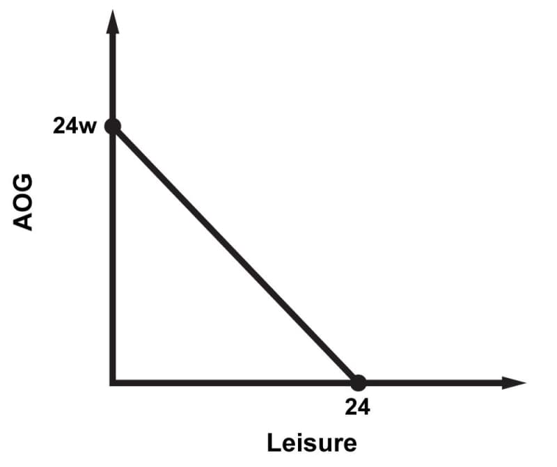
The indifference curves between leisure and all other goods would be similar to those we have seen in the goods and services market. We can combine a worker's budget constraint with his indifference curves to see how the worker would optimize the labor-leisure choice. With normally shaped indifference curves, the utility-maximizing choice represents (unsurprisingly) a mix of leisure and goods-consumption.

Change in Wage
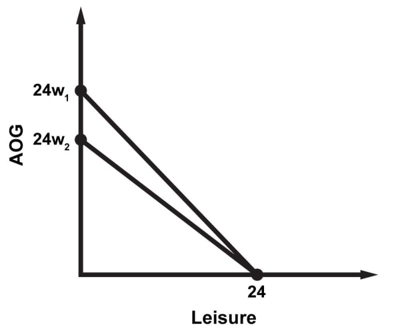
Just as a buyer's budget constraint pivots with a change in the price of one good, a worker's budget constraint can pivot with a change in the wage. If the wage increases, the budget line pivots outwards. If the wage drops, then the budget pivots inwards. Note that the maximum leisure point is fixed, since there are always 24 hours in a day. In the graph below, you can see the inwards pivot that occurs when the wage level drops: workers cannot afford as many other goods as they could prior to the drop in pay.
The substitution effect and the income effect, which we learned about in the chapter on Demand, also influence worker's decisions between consumption and leisure. When the wage increases, the income effect makes workers feel wealthier and therefore makes them want more of both leisure and consumption—more vacation time and also more “stuff.” The substitution effect, however, makes leisure more expensive, because the worker has to give up more wages for every hour spent in leisure. Think of the wages lost as the opportunity cost of leisure. So by the substitution effect, workers will want more consumption and less leisure—less vacation time and lots more stuff.
Therefore, when wages increase, the combined effect of the substitution and income effects is that workers will choose more consumption, but the effect on the level of labor and leisure is uncertain. If we assume that the substitution effect is stronger, then workers will choose to work more and play less, which makes sense, since a higher wage would give workers more incentive to work.

Is this always true that the substitution effect outweighs the income effect? Some economists believe that it is initially true, at relatively low wage levels. That leads to a labor supply curve with a familiar shape, sloping upward to indicate a willingness to work more as wage goes up. However, as the wage gets progressively higher, economists believe that eventually the income effect begins to outweigh the substitution effect, and very high wage-earners will begin to choose leisure over consumption even if their wage increases. Maybe that's why corporate bigwigs have the reputation of having too much free time to gallivant around on tropical islands. In such cases, the labor supply curve terminates in a surprising hook at its upper end:

An individual's labor supply curve marks out the number of hours they are willing to work at different wages, the same way that a seller's supply curve marks out how much they are willing to sell at different prices. How do we find the aggregate labor supply curve? To find aggregate labor supply from many individual supply curves, use horizontal addition to combine all of the work that workers are willing to perform at each wage level, to form the aggregate labor supply curve.