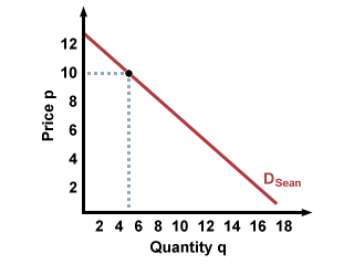
Instead of modeling demand graphically, we can model it using equations, known as demand equations or demand functions. While these equations can be very complex, we will use simple algebraic equations that correspond to the straight, downward-sloping lines we have been looking at. Just as the graphs provide a visual guide to consumer behavior, demand functions provide a numerical guide. For example, suppose Sean's demand curve for T-shirts looks like this.

The corresponding equation that describes Sean's demand for T-shirts is simply the equation for the line on the graph:
\(q = 25 - 2p\)
Note that \(q\) is described as a function of \(p\). If we want to see how much Sean will buy if the price is $10, we plug 10 in for \(p\) and find \(q\). In this case, because \(25 - (2\times10) = 5\), we conclude that Sean will buy 5 T-shirts.
When we want to find market demand using the algebraic approach instead of the graphical approach, we just add the demand equations together. So, if we're adding Sean's demand to Noah's demand, and Noah’s demand is given by \(q = 40 - 3p\), then the process for finding the market demand looks like this:
\(q = 25 – 2p\)
+ \(q = 40 – 3p\)
–––––––––––
\(q = 65 – 5p\)
If the price of a shirt is still $10, we find that together, Sean and Noah together will buy \(65 - (5\times10) = 15\) T-shirts.
One caveat: This method only works when each equation individually will result in a non-negative demand quantity. Suppose the price of a T-shirt is $13. Then Sean will supposedly want to buy \(25 - (2\times13) = -1\) shirt, while Noah will buy \(40 - (3\times13) = 1\) shirt, for a total of 0 T-shirts. In reality, Sean will buy 0 shirts and Noah will buy 1, for a total of 1 T-shirt. Always check that there will be no negative demand for the given price before adding equations together.


