


Aggregate supply represents the total supply of goods and services in an economy. However, the graphical analysis gets a little more complicated than for aggregate demand. The axes are the same, but for aggregate supply there are two curves, not just one: a curve for the short run and a curve for the long run.
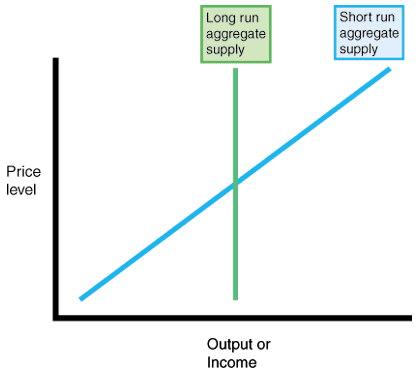
The short run aggregate supply curve is upward-sloping, while the long run aggregate supply curve is vertical.
Aggregate Supply in the Long Run
Why would aggregate supply be vertical in the long run? First, recall from the Growth chapter that output is a function of land, labor, and capital—the inputs to production. The amount of land is essentially constant. Thus, in the long run, an economy’s output level is a function of the amounts of labor and capital. The only way to increase output in the long run is to increase the levels of those inputs, or to raise their efficiency through advances in technology. That is, either the labor force must grow or there must be an increase in capital stock, the result of investment. Therefore, in the long run, the aggregate supply curve is affected only by the levels of labor and capital and not by the price level. Thus, the long run aggregate supply is vertical with respect to the price level.
Aggregate Supply in the Short Run
If the price level doesn’t matter for aggregate supply in the long run, why does it matter in the short run? There are a number of explanatory models, but here we will concentrate on one: compared to the costs of outputs, input costs tend to be “sticky.” The prices of goods and services sold to consumers and to firms can generally be adjusted on fairly short notice. Gas stations have electronic signage that makes price changes especially easy. Sellers of other goods may have menu costs (as described in the Inflation chapter), but even they can raise (or lower) prices in a matter of weeks once the decision to do so is made.
Input costs, on the other hand, do not change so easily. In many industries, wages are set by contracts. That is, workers are paid based on relatively permanent pay schedules that are decided upon by management or unions, or both. If the price level rises, management will not be in a hurry to renegotiate a new contract that raises workers’ pay. Leases on buildings and equipment are similarly locked in a year at a time. So are many contracts with suppliers of parts and raw materials. All of these sticky input costs, coupled with relatively non-sticky prices on output, mean that when the price level goes up, every unit of producers’ output becomes more profitable. This incentivizes a higher output level (which involves hiring more workers and ordering more parts and raw materials), until input costs rise to catch up with output prices.
On the flip side, when the price level falls, sticky input costs, coupled with less-sticky output prices, mean that every unit of output becomes less profitable. This incentivizes a reduced output level (which involves laying off workers or reducing their hours, and ordering fewer parts and raw materials), until input costs fall to catch up with output prices. The bottom line is that in the short term, output rises and falls as the price level rises and falls. That is why the short run aggregate supply curve slopes upward.
What about shifts in aggregate supply? These are rarer and are usually—though not always—responses to shifts in aggregate demand. For that reason, shifts in aggregate supply will be discussed in the context of the aggregate demand–aggregate supply model.