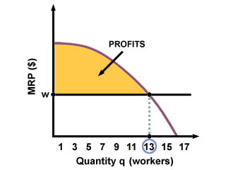
Aggregate Demand Curve for Labor
Just as we added all individual demand curves to find aggregate demand in the goods and services market, we use horizontal addition to add together all individual demand curves for labor to find the aggregate demand for labor. If you have equations representing different labor demand curves, simply add them together to find the new, aggregate demand. Graphically, add the quantities demanded at each wage level to generate a new labor demand curve. You can see how this is done in the Supply and Demand SparkNote.
Equilibrium in Labor Markets
Once you have generated aggregate supply and demand curves for labor, finding the market equilibrium, as with the goods and services market, is simply a matter of finding the intersection of the two curves (unless there is an artificial restriction on the market, such as a minimum wage). Let us consider two cases: an unrestricted labor market with shifts in the supply or demand curves, and a restricted market with a minimum wage.
Unrestricted Labor Market
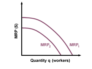
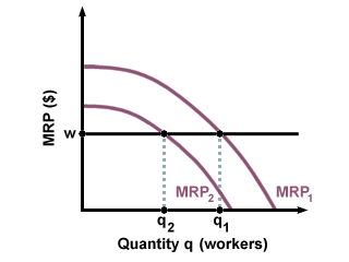
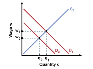
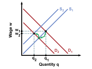
First, let us consider the market for hot chocolate when the price of marshmallows increases. Assuming that marshmallows and hot chocolate are complementary goods, the rise in the price of marshmallows causes a drop in the demand for hot chocolate. When demand for hot chocolate shifts in (drops), the price of hot chocolate falls. This drop in the price of hot chocolate lowers the MRP of every worker in the hot chocolate industry.
Why is this the case? Say that Charlie the hot chocolate maker can make 1000 packets of hot chocolate every day. If the price was originally $1 a packet, his MRP was $1000 a day. If the price falls to $0.75 a packet, Charlie can still only make 1000 packets a day, and so his MRP has fallen to $750. MRP, remember, is equal to the price times the marginal product of each worker.
MRP = (P) x (MP)
Restricted Labor Markets
What happens when the labor market is restricted in some way? Recall the case in the goods and services market where the government installs artificial limits on the market, such as taxes, price ceilings, or price floors. The government does similar things in the labor market, as well. Workers pay income taxes on their wages, and firms are required to pay no less than a regulated minimum wage for the labor they demand. These restrictions cause distortions in the way that the labor market works.
For instance, the U.S. runs on a progressive income tax system: for the first chunk of money you make, you pay no taxes, so you get to take home every penny that you earn. For the second chunk of money, you pay some taxes, so your take- home pay is a little lower. For your third chunk of money, the tax is a little higher, and so on. This means that the first $1000 that you make is actually $1,000, so you work for exactly the amount of money that you make. If you make $10,000, you pay some taxes, but not too much, so your take-home pay is almost the same as the amount of money that you earn. If you make $1,000,000, however, you pay a high marginal tax rate so that you might pay $0.40 in taxes on the last dollar you earn, meaning for that final dollar you put in $1 of work and got $0.60 in take-home pay. The effect of this is that as workers earn more and more money, they have less and less incentive to work: partly because they may feel that they have enough money, and partly because they have to work just as hard to get less money.


 payment page


