The Algebraic Approach
As with demand, it is also possible to model supply using equations. These supply equations, or supply functions, are used to numerically represent firm behavior and the variation of firm behavior with price. For simplicity's sake, we will again use simple algebraic equations.
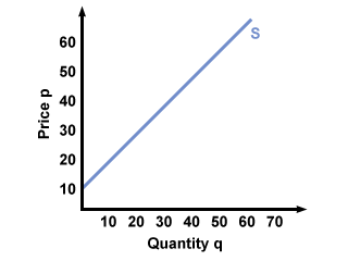
If Amy's bookstore sells textbooks with a supply curve that looks like this:

Q = -10 + PIf we want to see how many books the store is willing to sell if the price is $50, we plug 50 in for P and solve for Q. In this case,
Q = [-10 + 50] = 40 textbooksIf we want to solve for aggregate supply using the algebraic approach instead of the graphical approach, we just add the supply equations together. So, if we're adding Amy's bookstore's supply to Tony's bookstore's supply, it will look like this:

Q = [-15 + 2.5(50)] = 110 textbooks
One caveat: It is possible that some supply functions will sometimes give a negative quantity for some prices. For instance, the supply equation for Amy's bookstore will give a negative quantity supplied if the price is under $10 per textbook. Since it is impossible to supply a negative quantity of textbooks, for values under $10 the store will not sell any textbooks. Before adding together two or more supply equations, always check to make sure that none of them will give you negative results for the price for which you are solving.
To find the reservation price when working with supply functions, set Q equal to 0 and solve for P. The reservation price will be marginally higher than P when Q is equal to 0. For instance, if we want to find Amy's reservation price:
Q = -10 + PAmy's reservation price will be marginally higher than $10. Assuming that she can only sell whole books (that is, she can't sell 1/2 of a book), then her reservation price will be the price when her supply quantity will be 1:
0 = -10 + P
P = 10
1 = -10 + P
P = $11 per textbook
If we want to see how supply can change even without a change in the market price, we need to look at utility. While buyers get their utility from their preferences and needs, firms get their utility from profit. Basically, profit is how much a seller actually gains by making a sale (and what we use to measure how happy the seller will be), and is derived by subtracting the costs from income. The simplest form of the profit equation is as follows:
Profit = Total Revenue (TR) - Total Cost (TC)For instance, if an ice cream store pays $500 in rent, $500 in wages, and $200 for ice cream each month, and they sell 500 ice cream cones at $3 each, then their profit each month is:
[(500)(3) - (500 + 500 + 200)] = $300.One thing that can change their profit margin is the price. We know from before that changes in price are reflected in movements along one supply curve. However, changes in their costs, such as rent, wages, or gallons of ice cream can cause their supply curve to shift, since any of these changes would affect their willingness to sell ice cream at a given price.
We can see how this works when we change how much rent the ice cream store has to pay each month without changing the price they charge for an ice cream cone. If the monthly rent increases to $600, and nothing else changes, then their monthly profits will fall to $200. If you were the ice cream store owner, and you had this happened to you, how willing would you be to sell ice cream cones? Last month, you sold 500 cones and made $300. This month, you would have to work just as hard to make less money. It is easy to see why firms can be affected by more than just the price of a good when deciding how much to sell, and it is these considerations that can cause shifts in their supply curves.


 payment page


