


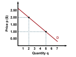
We have been looking at how changes in price can affect buyers' decisions: when price increases, demand decreases, and vice versa. However we have been assuming that when the price changes, all else is staying the same; this restriction allows us to use the same demand curve, with changes in demand being represented by movements up and down the same curve. This model of a buyer moving up and down one demand curve is correct if the only thing that is changing is the price of the good. If preferences or income change, however, the demand curve can actually shift.
For example, let's say that Conan's initial demand curve for concert tickets looks like curve 1. If Conan gets a new job, with a permanently higher income, however, his demand curve will shift outwards, to curve 2. Why is this? Conan realizes that he has more money, and that, as long as he doesn't lose his new job, he will always have more money. That means that he can buy more of what he likes, and he will have a higher demand curve for all normal goods.
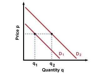
Note that for any price level, Conan's demand is now higher than it was before the demand shift. This can also occur with a change in buyer preferences. If Conan suddenly decides that he wants to collect jazz CDs, and he now likes jazz CDs much more than he did before, his demand curve will shift outwards, reflecting his new appreciation of jazz, and his willingness to pay more for the same CDs, since they have become more valuable in his eyes. Shifts in demand curves are caused by changes in income (which make the goods seem more or less expensive) or changes in preferences (which make the goods seem more or less valuable).
The Algebraic Approach
It is also possible to model demand using equations, known as demand equations
or demand functions. While these equations can be very complex, for now we will
use simple algebraic equations. We have been showing demand as straight,
downward-sloping lines, which can easily be translated into mathematical
equations, and vice versa. Just as the graphs provide a visual guide to
consumer behavior, demand functions provide a numerical guide to consumer
behavior. For example, if Sean's demand curve for T-shirts looks like this:
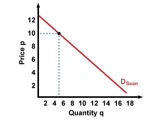
Q = 25 - 2PIf we want to see how much Sean will buy if the price is 10, we plug 10 in for P and solve for Q. In this case, [25 - 2(10)] = 5 T-shirts. When we want to find aggregate demand using the algebraic approach instead of the graphical approach, we just add the demand equations together. So, if we're adding Sean's demand for T-shirts to Noah's demand for T-shirts, it looks like this:
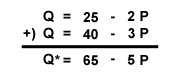
[65 - 5(10)] = 15 T-shirts.
One caveat in this method is that you can only add the equations together when both will result in positive demand. For example, if the price of a T-shirt is $13, Sean would supposedly want to buy [25 - 2(13)] = -1 T-shirts. Obviously that is impossible, and Sean will buy 0 T-shirts. But because Sean's demand equation would yield the answer –1, adding the demand equations together would result in a wrong answer. When using this method, always check to make sure that there will be no negative demand for the given price before adding equations together. To find how many T-shirts Sean and Noah would buy in this case, you would only look at Noah's demand,
[40 - 3(13)] = 1 T-shirt.